An improved stochastic averaging process on a monostable piezoelectric vibrational energy harvester model excited by colored noise

1. Introduction

In recent years, accumulating attention has been paid to the piezoelectric vibration energy harvesting (VEH) systems due to their capability of collecting the ambivalent background energy, which is usually free. Mathematical analysis on this topic is of great importance. One type of well-known vibration energy harvesting system, which is used to model a basally excited cantilever with piezoelectric ceramic layers attached to it, is displayed in the form:

The Eq. (1) and Eq. (2) describe the relation of motion states and piezoelectric voltage, where $w$ denotes the relative displacement of mass $m$, ${\ddot{w}}_b$ denotes the basal acceleration, $c$ denotes the linear damping coefficient, $U\left(w\right)$ denotes the potential energy of the conservative part of the mechanical subsystem, $V\left(\tau \right)$ denotes the output voltage across the equivalent resistive load $R$, $C_p$ is the piezoelectric capacitance, $\beta$ denotes electro-mechanical coupling coefficient, the dot represents the derivative with respect to time $\tau$.

Introduce the non-dimensional parameters:

where $k_1$denotes the linear stiffness coefficient of the conservative part $dU\left(w\right)/dw$, $L$ denotes a chosen character length, $t$ presents the dimensionless time, $T$ denotes the character time scale$\sqrt{m/k_1}$, $x$ denotes the dimensionless displacement, $\mu$ denotes the linear dimensionless damping coefficient, $\eta \left(t\right)$ denotes the dimensionless basal acceleration. The Eq. (1) and Eq. (2) can be transformed to as follows:

where, the expression $f\left(x\right)$ presents the combination of dimension less linear and nonlinear stiffness terms, i.e.$f\left(x\right)=dU\left(x\right)/dx$. Based on this model, plenty of researches have been carried out. When $f\left(x\right)={\omega }_0^{2}x+\alpha x^3$ ($\alpha >$0), Eq. (3) is a duffing type (mono-stable) VEH [1-3], where ${\omega }_0$is the dimensionless linear frequency, $\alpha$ denotes the dimensionless nonlinear stiffness coefficient. When $f\left(x\right)={\omega }_0^{2}x+\alpha x^3$ ($\alpha <$0), Eq. (3) is called the bi-stable (double well) VEH [4]-[7]. When $f\left(x\right)={\omega }_0^{2}x-{\alpha }_1{x}^3+{\alpha }_2{x}^5$ and $f\left(x\right)=0$ has five real roots, Eq. (3) is called the tri-stable VEH [8]-[10]. When $f\left(x\right)$ has much complex expressions, there even exists quadruple well VEH [11], [12] However, one should notice that the early researches were based on harmonic excitation, which could hardly simulate the noise in real-world. As the research deepens, a better method is in need for the research of VEH.

Daqaq [13], [14] applied the moment method based on the Fokker- Planck-Kolmogorov (FPK) equation to study a duffing type and a bi-stable VEH driven by white noise as well as colored noise. One striking conclusion was proposed: the mean square output voltage and the output power are proportional to the white noise density but have no relation with the nonlinear stiffness coefficient, i.e., the response of a white noise excited bi-stable VEH has no relation with the shape of the potential well. But Daqaq and He [15] found that the moment method could lead to large errors and even wrong predictions when the potential wells are deep enough. Similarly, Chen and Jiang [16] using the moment method, studied a VEH model with order-2 and order-4 nonlinear stiffness terms subject white noise. By then, one could find that the nonlinear stiffness term did have an influence on the responses. Subsequently, Chen and Jiang [17] applied an equivalent linearization technique to study a white noise excited VEH model with cubic nonlinearity. In their paper, the influence of the nonlinear stiffness was approximately simplified to be disturbing terms to the linear stiffness term and the linear damping term. Then, the two disturbing terms were obtained by the minimal mean square error principle.

Stochastic averaging method is another popular method in studying the randomly excited VEH for it can give the approximate probability density functions of different random variables. Chen and Jiang [18] applied the standard stochastic averaging method to solve some different types of VEH subject to white noise. In this paper, the displacement and velocity are assumed to be $x=A\mathrm{c}\mathrm{o}\mathrm{s}\theta$, $\dot{x}=-A{\omega }_0\mathrm{s}\mathrm{i}\mathrm{n}\theta$ (where $A$ denotes the transient amplitude and ${\omega }_0$ denotes the fundamental frequency). Although the influence of nonlinear stiffness on frequency is ignored, the method offers acceptable predications on condition that the nonlinearity is not strong. However, when the stiffness nonlinearity is strong, the standard stochastic averaging will lose its accuracy. Because, although nonlinear stiffness is taken into account during modeling, the stiffness nonlinear term will be eliminated in subsequent calculations. To solve this problem, Chen and Jiang [19] assumed the displacement and velocity in the form of $x=A\mathrm{c}\mathrm{o}\mathrm{s}\theta \text{,}$$\dot{x}=-A\omega (A,\theta )\mathrm{s}\mathrm{i}\mathrm{n}\theta$, where the frequency $\omega \left(A,\theta \right)$ is a so-called generalized harmonic functions, they obtained the averaged frequency $\omega \left(A\right)$ by integrating the $\omega (A,\theta )$ with respect to $\theta$. Liu et al. [20], Li and Xu [21], Xu and Wang [22] applied the energy envelope stochastic averaging method and assumed the frequency is the function of the total mechanical energy H. The similarity of the references [19] and reference [20]-[22]is that they all concerned the nonlinear stiffness term had an influence on the response frequency, so they used an energy determined frequency $\omega \left(H\right)$ and an amplitude determined frequency $\omega \left(A\right)$ instead of the fundamental frequency ${\omega }_0$. But both methods are very time-consuming, especially the second one. Because the explicit expression of the $\omega \left(H\right)$ must be obtained by ellipse integrals, which cannot be easily expressed as polynomials or a fraction.

In recent years, significant progress has been made in relevant research. In 2018, Fang Fei et al. [23] investigated a VEH model subjected to parametric and external excitations. They considered stiffness nonlinearity using the Hamiltonian principle and studied the effects of damping, load coefficient, electromechanical coupling coefficient, and excitation amplitude on the frequency response curve. In 2019, Wang Yaobin et al. [24] investigated the electromechanical response of a VEH and observed that during the process of increasing stiffness nonlinearity, the softening behavior of the system first increases and then decreases. They discovered an optimal value for the stiffness nonlinearity. In 2020, Xia Guanghui et al. [25] utilized the multi-scale method to investigate the response of a VEH with an additional mass block under parametric excitation and direct excitation. They found that with an increase in the mass block, the system's stiffness nonlinearity coefficient decreases, leading to a softening behavior in the amplitude-frequency response curve. In 2020, Zhang Yanxia [26] investigated the stochastic bifurcation of a three-well piezoelectric cantilever beam under colored noise excitation, varying the third-order stiffness term, fifth-order stiffness term, noise intensity, and correlation time as bifurcation parameters. The study revealed that noise intensity can enhance the generation of average output power, while correlation time leads to a reduction in average power generation. In 2021, Costa [27] conducted a parameter study on the third-order nonlinear stiffness coefficient in a bistable VEH system subjected to harmonic excitation. The results showed that higher linear stiffness coefficient and lower nonlinear stiffness coefficient lead to better power output performance.

Based on the above, the traditional stochastic averaging methods eliminate the stiffness nonlinearity coefficient in the subsequent calculation process, which significantly affects the computational accuracy. Although some scholars attempt to compensate for this using t the energy envelope stochastic averaging method, the calculation results are challenging to obtain, and the computational process becomes cumbersome. Indeed, in recent years, an increasing number of scholars have been paying attention to the significance of stiffness nonlinearity. Various studies have demonstrated that stiffness nonlinearity indeed plays a crucial role in influencing the system's response. In this paper, a mono-stable VEH model subject to colored noise is investigated. An approximate frequency $\omega \left(A\right)$ in polynomial form can be obtained by the energy balance method [28]. The $\omega \left(A\right)$ will have a concise and explicit expression. Based on the obtained frequency $\omega \left(A\right)$, a stochastic averaging method for strong nonlinearity is carried out. After that, the stationary probability density function (PDF) of the displacement, the joint probability density function of the displacement and velocity, as well as the mean square voltage are all given theoretically and numerically. The key issue of this paper is to make sure the approximate frequency $\omega \left(A\right)$ will maintain accurate prediction of the responses. Numerical simulations are carried out to verify the accuracy of this method.

2. The energy balance method

The mono-stable piezoelectric vibration energy harvester model (Duffing type) to be studied in this paper is as follows:

The stationary displacement, the velocity and the stationary voltage are assumed to be:

where $\theta =\mathrm{\Phi }\left(t\right)+\tau \left(t\right)$, $A$ is the transient amplitude, $\tau \left(t\right)$ is the random phase, $v(A,\theta )=d\mathrm{\Phi }/dt$ denotes the transient frequency.

Substituting Eq. (7) into Eq. (6) yields:

Then substitute Eq. (7) and Eq. (8) into Eq. (5), one has:

Thus, the total mechanic energy (Hamilton function) of the Eq. (9) is as follows:

When $\theta =$0° and $\theta =$45°, the energy $H$ equals to the following, respectively:

Obviously, when the energy dissipated by the damping can balance the noise input energy, there must exists $H_1=H_2$. One can solve out the to be determined frequency [28] as follows.

In view of that the dimensionless load coefficient $\gamma$ is much smaller than 1, we have ${\gamma }^2\ll {\nu }^2$, it is reasonable to assum $\vartheta \beta v^2/({\gamma }^2+v^2)\approx \vartheta \beta$, then one has the approximate frequency:

Letting ${\omega }^2={\omega }_0^2+\vartheta \beta$, finally one has:

In this section, an approximate frequency determined by amplitude $A$ is obtained. In the next section, this frequency will be used in the stochastic averaging procedure.

3. Stochastic averaging method

The stiffness term is defined as $f\left(x\right)={\omega }_0^{2}x+\alpha x^3$, the damping term is defined as $c(x,\dot{x})=\mu \dot{x}-\vartheta u\left(t\right)$. The nonlinear stiffness coefficient is assumed to be strong, while the damping $c(x,\dot{x})$ term is weak, Eq. (5) can be rewritten as:

Taking derivative to $x=A\mathrm{c}\mathrm{o}\mathrm{s}\theta$ with respect to time $t$ yields:

Eq. (17) can be simplified as:

Then, taking derivative to $y=\dot{x}=-Av\mathrm{s}\mathrm{i}\mathrm{n}\theta$ with respect to time $t$, yields:

In which one has:

Combining the Eq. (17) and Eq. (18) and taking Eq. (19) and Eq. (20) into account, one has a pair of stochastic differential equations:

The above pair of equations can be rewritten to be the standard form as:

where:

The Eq. (23) and Eq. (24) can be simplified to the Itô stochastic differential equation:

where $m\left(A\right)$ is the drift term while ${\sigma }^2\left(A\right)$ is the diffusion term, $W\left(t\right)$ is the standard unit Brown's motion. The expression of $m\left(A\right)$ and ${\sigma }^2\left(A\right)$ are given by the following formular:

where $⟨•⟩=\frac{1}{2\pi }{\int }_0^{2\pi }•d\theta$ is the averaging operator, $R_{ij}\left(\tau \right)$ is the correlation function.

The noise density is 2$D$, the time delay coefficient is $\lambda$, then $R_{ij}\left(\tau \right)$ has the form of:

where the operator $E\left[·\right]$ presents the mathematical expectation, while $\delta \left(\tau \right)$ is the Dirac-delta function.

The drift coefficient $m\left(A\right)$, and the diffusion coefficient ${\sigma }^2\left(A\right)$ are given as:

In which the coefficients are:

4. The stationary probability density functions

The averaged Fokker-Plank-Kolmogorov (FPK) equation associated with Itô Eq. (25) is of the form:

where $p\left(A,t\right)$ is the transition probability density of displacement amplitude $A$. Under assumption of $\frac{\partial p}{\partial t}=0$ the stationary solution of FPK equation $p\left(A\right)$ for Eq. (30) is of the form:

where constant $N$ is the normalization constant.

Substituting Eq. (28), Eq. (29) into Eq. (31) yields the stationary PDF of the equivalent amplitude:

The stationary probability density of total mechanic energy i.e., Hamiltonian function $H$ can be obtained as follows:

The transient amplitude is solved as:

The joint stationary probability density of displacement$x$and velocity $y=\dot{x}$ can be further obtained from $p\left(H\right)$ as follows:

where $T\left(H\right)$ is the average time period defined as $T\left(H\right)=2\pi /v\left(A\right).$

By integrating Eq. (35), the PDF of the displacement as well as the PDF of the velocity is obtained as Eq. (36) and Eq. (37):

The approximate relation with the electric voltage and the mechanical states in Eq. (8) is simplified to be the Eq. (37) by replacing $\nu$ by $\omega$:

Thus, the PDF of the electric voltage is obtained based on the Eq. (38):

The mean-square value of the electric voltage is also derived through the approximate relation Eq. (37):

5. Numerical simulations

The Monte Carlo method is applied to verify the effectiveness of the above theoretical predictions. The parameters in Eq. (5) and Eq. (6) are taken as: The parameters are set as: ${\omega }_0=$1, $\mu =$0.05, $\beta =$0.01, $\gamma =$0.1, $\vartheta =$ 0.05. The noise density $D$ is chosen as $D=$0.001 and $D=$0.002, and the time delay coefficient $\lambda$ is chosen as 0.3, 0.5 and 0.8, separately. In order to emphasis the accuracy of this method, even if the nonlinear stiffness coefficient $\alpha$ is significantly large, the coefficient $\alpha$ is set as 20 and 50 during the simulation, respectively. The numerical solutions of the oscillator Eq. (2) could be obtained by an order-2stochastic Runge-Kutta algorithm [29]. The numerical solutions were obtained using MATLAB. For each combination, totally 2,000 sets of colored noise are imposed the Eq. (5) and Eq. (6). Each set of noise includes 60,000 numbers. The time step is set as $\mathrm{\Delta }t=\text{0.005}$. The last 10,000 steps are kept as the stationary responses. Finally, doing statistic on total stationary $n=$2,000×10,000 values of $x$ and $u$, the stationary probability density function (PDF) of the displacement $p\left(x\right)$ and the voltage $p\left(u\right)$ is represented by a dot plot. The theoretical solutions obtained using Eq. (36) and Eq. (39) in Mathematica are represented using solid lines. The figure of the standard stochastic averaging method is sourced from reference [17] and is presented using dashed lines.

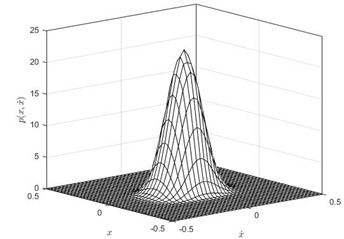
Fig. 1The analytical solution and numerical solution of stationary PDFs of electric voltage and displacement: a), b) D= 0.002, λ= 0.5, α= 20 and 50; c), d) λ= 0.5, α= 50, D= 0.001 and D= 0.002; e), f) α= 50, D= 0.002, λ= 0.3 and 0.8. a), c) e) PDFs of displacement, b) d, f) PDFs of voltage. Solid lines: improved method in this paper, see Eq. (36) and Eq. (39); dashed lines: standard stochastic averaging method in reference [17]; dots: numerical simulation)

a)

b)

c)

d)

e)

f)

In Fig. 1, due to the fact that the standard stochastic averaging method will eliminate the nonlinear stiffness coefficient $\alpha$ during the averaging process, one can see clearly that the standard stochastic averaging method exhibits significant errors when compared to the numerical solutions, and these errors increase as the stiffness nonlinearity becomes larger. However, the improved stochastic averaging method manages to maintain accurate predictions even when the stiffness nonlinearity is relatively large. Also, the larger the coefficient $\alpha$ becomes, the higher peak values and smaller range of the PDF value it will result in. Furthermore, one should also notice that even if the frequency $\nu \left(A\right)$ (see Eq. (14)) which is used in this method has very concise form, this form still offers very good accordance of the theoretical prediction and the numerical simulation. The Fig. 1. also indicates that the improved method offers good accuracy with the time delay coefficient $\lambda$ ranging from 0.3 to 0.8. And the larger $\lambda$ will lead to the larger range of motion.

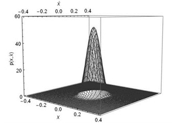
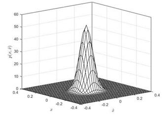
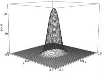
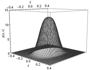
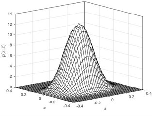
Fig. 2The joint Stationary PDF of displacement x and velocity y: a), b) for D= 0.002, λ= 0.3, λ= 50; c), d) for D= 0.002, λ= 0.5, α= 50; e), f) for D= 0.002, λ= 0.8, α= 50; a), c), e) are given by Eq. (35); b), d), f) are numerical simulation

a)

b)

c)

d)

e)

f)

Subsequently, the joint PDF of displacement $x$ and velocity $y=\dot{x}$ are numerically simulated. In this part, the parameters are set as: ${\omega }_0=$1, $\mu =$0.05, $\beta =$0.01, $\gamma =$0.1, $\vartheta =\text{0.05}$, $D=$0.002, $\alpha =$50. The time delay coefficient $\lambda$ is chosen as 0.3, 0.5 and 0.8, separately. The numerical solutions were obtained using MATLAB. We take 40×40 grids in a range $\left\{-0.4\le x\le 0.4,-0.4\le y\le 0.4\right\}$ with a space gap:$\mathrm{\Delta }x=\mathrm{\Delta }y=\text{0.02}$. Then we count the numbers $n_{ij}$ ($i$, $j=$1-40) of the $n=$2,000 ×60,000 stationary $\left(x,y\right)$ dots which fall within each grid. Finally, the joint PDF $p\left(x,y\right)$ value of each grid can be calculated out by $p(x_i,y_i)=n_{ij}/(n\times \mathrm{\Delta }x\times \mathrm{\Delta }y$). The theoretical solutions obtained using Eq. (32) and Eq. (35) in Mathematica. The joint PDFs are illustrated in Fig. 2. Fig. 2 shows that the theoretical predication on the joint probability density function of the displacement and velocity coincides with the numerical simulation.

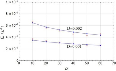
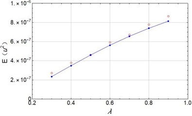
Finally, the mean square value of the electric voltage $E\left(u^2\right)$ is predicted by the Eq. (40) and is numerically simulated. The Fig. 3(a) shows the results with the nonlinear stiffness coefficient $\alpha$ ranging from 10 to 60. When noise density $D$ is chosen as 0.001 and 0.002, the Eq. (39) offers good accordance with the numerical simulation. Fig. 3(b) shows the good prediction $E\left(u^2\right)$ with time delay coefficient $\lambda$ ranging from 0.3 to 0.9. When $\lambda$ is larger than 0.8, the error becomes visible. It is obvious that the larger nonlinear stiffness coefficient $\alpha$ will lead to smaller mean square value of the electric voltage. While, larger time delay coefficient $\lambda$ will result in larger $E\left(u^2\right)$.

Fig. 3Mean square voltage changes with system parameters: a) D= 0.001 and 0.002, λ= 0.5; b) D= 0.002, α= 50; Dotted lines: theoretical prediction by Eq. (40); circles: numerical simulation)

a)

b)

6. Conclusions

In this paper, an improved stochastic averaging method is introduced, the energy balance method has been employed to derive a concise expression of the transient frequency $\nu \left(A\right)$. The improved method significantly reduces computation time. Comparing with the standard stochastic averaging method, the improved method, considering the stiffness nonlinearity, demonstrates a notable improvement in predictive accuracy under colored noise excitation. The results are as follows:

1) This improved method has good accuracy in predicting the PDFs of the VEH system even if the expression of $\nu \left(A\right)$ is short. This method can get rid of the disadvantage of large time consuming in calculating $\omega \left(H\right)$ in references [19], [20]-[22].

2) The nonlinear coefficient $\alpha$ does have an influence on the PDFs of displacement and electric voltage. Larger $\alpha$ will result in smaller motion range, higher peak of PDFs and smaller mean square value of the voltage. Even if the $\alpha$ is considerably large, this improved method maintains good accuracy.

3) Larger time delay coefficient $\lambda$ will lead to larger motion range and larger mean square value of the voltage.

The improved stochastic averaging method introduced in this paper contributes to enhancing the output performance of piezoelectric transducers and deepens the understanding of the response patterns of single-steady-state models under random excitation.